Visualizing and animating a swarm
Visualization is turboswarm's top priority. This tutorial records a run and
turns it into a convergence curve, a variant comparison, and an animation of the
swarm moving over the objective landscape.
Visualization uses Matplotlib (a core dependency), so there is nothing extra to install.
Record the run
Plots and animations need the per-iteration history, which is recorded by
default (record_history=True). We optimize the 2-D
Rastrigin function — a classic multimodal test case.
import turboswarm as pso

bounds = [(-5.12, 5.12)] * 2
result = pso.minimize("rastrigin", bounds=bounds, seed=3, max_iter=60)
print(f"{result.best_value:.3e}")     # 8.286e-06  (optimum is 0)
Plot convergence
viz.plot_convergence draws the global best value per iteration (log scale by
default):
Compare variants on one chart
Run the same problem with different velocity rules and overlay their curves — this is the quickest way to see which variant converges fastest:
runs = {
    v: pso.minimize("rastrigin", bounds=bounds, velocity=v, seed=3, max_iter=60)
    for v in ["inertia", "constriction", "fips"]
}

ax = None
for name, r in runs.items():
    ax = pso.viz.plot_convergence(r, label=name, ax=ax)
ax.set_title("Convergence by velocity variant (rastrigin, 2D)")
plt.show()

for name, r in runs.items():
    print(name, f"{r.best_value:.3e}")
# inertia       8.286e-06
# constriction  4.412e-03
# fips          4.692e-07
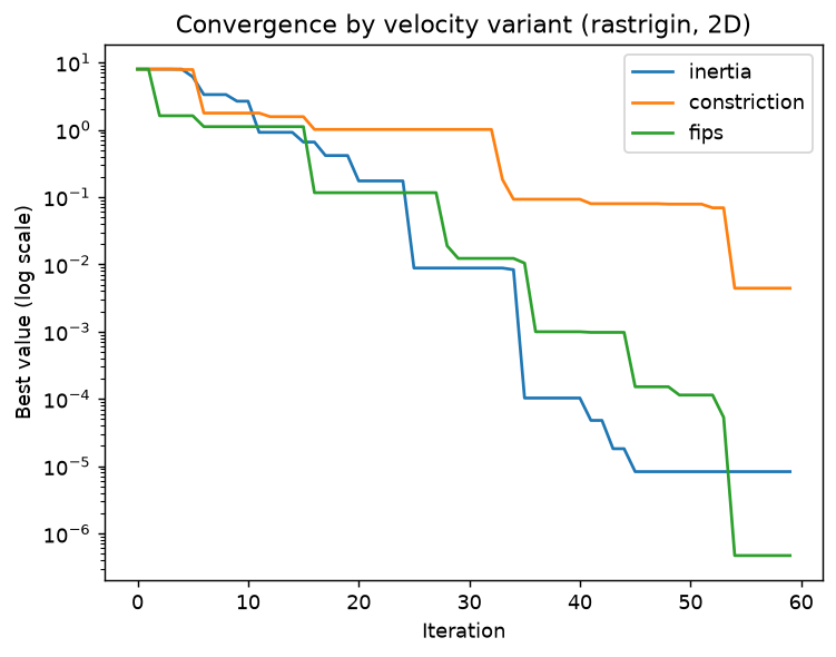
On this problem and seed all three reach the optimum region; fips and
inertia get closest. Comparing variants under identical conditions like this
is exactly what the library is designed for.
Animate the swarm
For 2-D problems, viz.animate_swarm draws the particles moving over a contour
of the objective. It returns a Matplotlib animation you can display in a
notebook or save to a file:
anim = pso.viz.animate_swarm(result, "rastrigin", bounds)
anim.save("swarm.gif", fps=10)        # or display it inline in a notebook
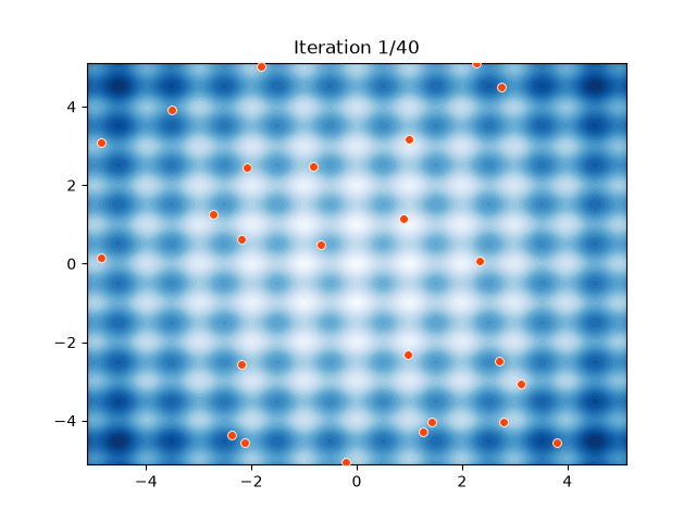
The particles start scattered and contract toward the global optimum at the origin as the iterations progress.
Note
animate_swarm supports 2-D problems and needs record_history=True
(the default). For higher dimensions, plot convergence instead, or project
to two dimensions before animating.
A 3D view of the landscape
For a more striking picture, render the objective as a 3D surface and drop the
final swarm onto it with plot_surface:
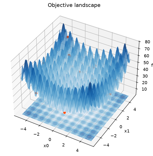
pso.viz.animate_swarm_3d(result, pso.benchmarks.rastrigin, bounds) animates the
swarm flying over this surface, with the best-so-far marked by a gold star and a
slowly rotating camera — see the Visualization guide.
Next steps
- For multi-objective runs,
viz.plot_paretodraws the trade-off front. - To study how hyperparameters affect results, see
Sensitivity analysis and
viz.plot_sensitivity.